(This analysis was written at the same time I was writing the code and deciding how I should proceed. I have already read too many data analysis posts that give the final, correct and beautiful answer, and don't show all the problems encountered along the way. So, except for a very initial part that I had already done (basically the XML data loading), all you will read below is following my train of thought at that precise moment. Here we go.)
Bixi is the name of Montreal's municipal bike rental service. It runs approximately between April 15th and November 15th each year and hundreds of Montrealers use it during the time it's active. Through their website, they offer XML data regarding the status of each of their bases (location, number of available bikes, number of free spots, etc). I decided to get some data during last year to play around with it when I had the time, which was now.
This script below was running every 30 minutes on my hosting machine (DreamHost, in case anyone is interested) between September 17th and December 14th:
cd /home/chema/bixidata &&
wget https://montreal.bixi.com/data/bikeStations.xml -q -O $(date +\%Y-\%m-\%d_\%H:\%M:00).xml
As you can see, nothing extremely fancy. It took me a while to learn that you must escape the % char inside of a cron job, but here we have it. This will download the current status XML file and store it in a file that contains the precise date we downloaded it.
As you read above, Bixi runs until November 15th approximately. Why did I run the script until mid-December? Well, I forgot to stop it.
The XML structure contains a number of nodes, of which I am keeping the following:
id: just a numerical identifier for that station.name: a string with the station name (e.g. "Notre Dame / Place Jacques Cartier")lat,long: latitude and longitude for that station.nbBikes: number of bikes available in that station at that moment.nbEmptyDocks: number of free spots available in that station at that moment.latestUpdateTime: the last time the information above was updated by the station.lastCommWithServer: the last time the information above was communicated to the server.
Here's the function that reads the whole thing:
library(XML)
processXMLFile <- function(file) {
    cat("Processing", file, "...")

    # Some XML is malformed, so let's try to catch that right at the beginning
    tryCatch({
        # If there is an error, it will be triggered by this line
        xml <- xmlParse(file)
        latestUpdateTime <- xpathSApply(xml, path = "//station/latestUpdateTime", xmlValue)
        if (length(latestUpdateTime) == 0)
            latestUpdateTime <- NA

        lastCommWithServer <- xpathSApply(xml, path = "//station/lastCommWithServer", xmlValue)
        if (length(lastCommWithServer) == 0)
            lastCommWithServer <- NA

        # Obtain date from the file name
        datepart <- strsplit(file, "/|\\.", perl = TRUE)[[1]][7]
        datepart <- as.POSIXct(datepart, format = "%Y-%m-%d_%H:%M:%S")

        res <- data.frame(id = as.numeric(xpathSApply(xml, path = "//station/id", xmlValue)),
                          name = xpathSApply(xml, path = "//station/name", xmlValue),
                          lat = as.numeric(xpathSApply(xml, path = "//station/lat", xmlValue)),
                          long = as.numeric(xpathSApply(xml, path = "//station/long", xmlValue)),
                          nbBikes = as.numeric(xpathSApply(xml, path = "//station/nbBikes", xmlValue)),
                          nbEmptyDocks = as.numeric(xpathSApply(xml, path = "//station/nbEmptyDocks", xmlValue)),
                          latestUpdateTime = as.numeric(latestUpdateTime),
                          lastCommWithServer = as.numeric(lastCommWithServer),
                          filedate = datepart,
                          stringsAsFactors = FALSE)
        cat("\n")
        return(res)
    },
        error = function(cond) {
            message("ERROR! Skipping file")
            return(NULL)
        }, warning = function(cond) {
            message("Warning! Skipping file")
            return(NULL)
        }
    )
}
Does it have to be so convoluted? Well, yes. A very first version I wrote (just some minutes before I decided to write the whole thing as I was doing it) didn't use the tryCatch block at all. However, some of the XML files contained malformed information that caused the whole thing to crash. I had to add both the error and the warning calls (this last one was probably never used, but anyway); in those cases I am returning NULL: as I am using this function within a lapply loop, these values will be discarded. And therefore:
XMLPATH <- "/home/chema/tmp/bixi/"
# Read all data into a single data.frame
cachefile <- "data/bixi.Rda" # and don't do it every time I run it
if (!file.exists(cachefile)) {
    datafiles <- dir("/home/chema/tmp/bixi/", pattern = "xml", full.names = TRUE)
    # We can skip some obviously wrong files by looking at the size
    sizes <- sapply(datafiles, function(x) file.info(x)$size)
    datafiles <- datafiles[sizes > 100000]
    # Now read the files using the XML function
    bixi <- lapply(datafiles, processXMLFile)
    bixi <- do.call(rbind, bixi)
    save(bixi, file = cachefile)
} else {
    load(cachefile)
}
This is a lengthy process, and my laptop (an old Dell purchased in 2007 that has suffered more than I dare to tell) took several minutes to finish it, that's why I am storing the final result and re-loading it every time I load the script.
To make sure I understood the meaning of latestUpdateTime and lastCommWithServer, I plotted one against the other and added a blue identity line (intercept = 0, slope = 1), resulting in this:
plot(bixi$latestUpdateTime, bixi$lastCommWithServer,
     main = "latestUpdateTime and lastCommWithServer",
     xlab = "latestUpdateTime", ylab = "lastCommWithServer",
     pch = 19, col = rgb(0, 0, 0, 0.2))
abline(a = 0, b = 1, col = "blue")
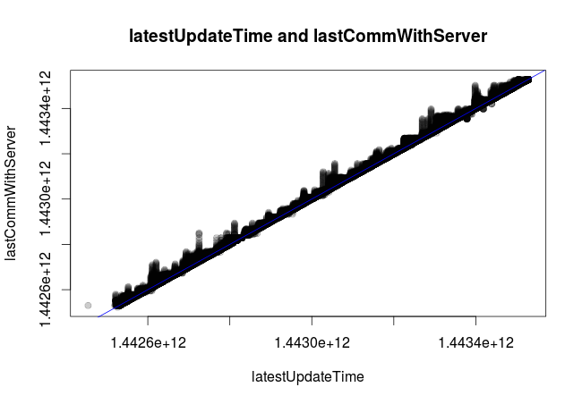
So it looks like the bases can update their stats at any given moment, but they do not necessarily update that information before sending it to the logging server. I therefore will consider latestUpdateTime as the real time. Note that I still have not converted the UNIX timestamps to a proper date format. Let's do it now.
# Convert to proper dates
bixi$latestUpdateTime <- as.POSIXlt(bixi$latestUpdateTime,
                                    origin = "1970-01-01")
bixi$lastCommWithServer <- as.POSIXlt(bixi$lastCommWithServer,
                                      origin = "1970-01-01")
head(bixi[, c("latestUpdateTime", "lastCommWithServer", "filedate")])
      latestUpdateTime   lastCommWithServer            filedate
1 47681-12-15 11:29:36 47681-12-18 22:12:51 2015-09-17 16:00:00
2 47681-12-11 17:59:44 47681-12-18 15:48:04 2015-09-17 16:00:00
3 47681-12-22 12:59:58 47681-12-22 12:59:40 2015-09-17 16:00:00
4 47681-12-21 02:51:47 47681-12-21 03:00:55 2015-09-17 16:00:00
5 47681-12-22 06:20:00 47681-12-22 06:42:19 2015-09-17 16:00:00
6 47681-12-10 20:46:54 47681-12-18 15:31:46 2015-09-17 16:00:00
Great Scott! This... is obviously not right. latestUpdateTime and lastCommWithServer are in milliseconds. Let's correct that:
# Convert to proper dates
bixi$latestUpdateTime <- as.POSIXlt(bixi$latestUpdateTime / 1000,
                                    origin = "1970-01-01")
bixi$lastCommWithServer <- as.POSIXlt(bixi$lastCommWithServer / 1000,
                                      origin = "1970-01-01")
head(bixi[, c("latestUpdateTime", "lastCommWithServer", "filedate")])
     latestUpdateTime  lastCommWithServer            filedate
1 2015-09-17 18:47:32 2015-09-17 18:52:30 2015-09-17 16:00:00
2 2015-09-17 18:42:10 2015-09-17 18:52:07 2015-09-17 16:00:00
3 2015-09-17 18:57:43 2015-09-17 18:57:43 2015-09-17 16:00:00
4 2015-09-17 18:55:40 2015-09-17 18:55:40 2015-09-17 16:00:00
5 2015-09-17 18:57:19 2015-09-17 18:57:20 2015-09-17 16:00:00
6 2015-09-17 18:40:54 2015-09-17 18:52:06 2015-09-17 16:00:00
We're almost there, but not quite yet. There seems to be an offset of around 3 hours between the latestUpdateTime and the filedate information that I wrote on the file name. Of course, I want my times to reflect the Montreal time zone, but the DreamHost server is on PST, which is exactly 3 hours less. That can be easily corrected:
# Time zone correction
bixi$filedate <- bixi$filedate + 3 * 60 * 60 # time operations are in seconds
I won't write the output of the head command again so as not to bore you, but everything looks OK now, we can proceed.
Also, while exploring these values I ran a global summary on the full dataset and I noticed that some entries have lat or long set to 0, which does not make any sense (for Montreal, that is). Let's fix that too. Note: I will not try to correct any missing or corrupted data. When in doubt, I will simply drop the whole thing. Like now:
# Remove incorrect latitude and longitude
bixi <- bixi[bixi$lat != 0 & bixi$long != 0, ]
I want to have the data for every base sampled at the same time points, so I don't have to care about this anymore. That's why I was storing the XML file with the time stamp in its name. That way, I can retrieve it in the XML reading function and return it as just another field in my data.frame object: filedate. I am going to use the latestUpdateTime for each base and I will do a simple linear interpolation to estimate how many bikes / free spots where there at filedate. I first want to check if these sampling times are too far apart. I begin with something simple:
mean(bixi$filedate - bixi$latestUpdateTime)
Time difference of NA secs
That's... weird. I forgot to do a summary before converting the time stamps, and I know I am returning NA if any of them does not exist in the XML file (I was getting early errors due to this). I re-check:
sum(is.na(bixi$latestUpdateTime))
[1] 807180
This is not good at all. More than 86 % of my samples did not come with a proper time stamp. I checked some XML files chosen at random and yes: the nodes are simply not there.
There are few options here, so I go for the quickest one: I will use the time when I saved the file to disk and be done with it. There is a useful lesson here: be a bit redundant when retrieving data, it might save your ass later.
Also, there is something fishy going on with the number of bikes and free spots:
> sum(bixi$nbBikes + bixi$nbEmptyDocks == 0)
[1] 35838
So in some cases it seems that there were neither bikes nor free slots in certain bases. I will also drop that from the dataset.
# Remove cases with no bikes and unused columns
bixi <- bixi[bixi$nbBikes + bixi$nbEmptyDocks > 0, ]
bixi$latestUpdateTime <- NULL
bixi$lastCommWithServer <- NULL
Ok, now: let's get two full months of data. We can get, for instance, from September 21st to November 23rd. We begin a Monday and end a Sunday.
# Subset by date
bixi <- bixi[bixi$filedate >= as.POSIXct("2015-09-21 00:00:00 EDT") &
             bixi$filedate < as.POSIXct("2015-11-23 00:00:00 EDT"), ]
Now it would be interesting to see if we have complete datasets for all the stations in this time period. We can use the excellent package dplyr for this, or we can have also use the base function aggregate. I'll go with the first option:
n_stations <- bixi %>% group_by(name) %>% summarise(n = n())
n_stations
Source: local data frame [453 x 2]

                         name     n
                        (chr) (int)
1         10e Avenue / Masson  1471
2       10e Avenue / Rosemont  1471
3  12e Avenue / Saint-Zotique  1470
4        15e Avenue / Laurier  1471
5         16e avenue/Rosemont  1471
6             18e av/beaubien  1471
7   18e Avenue / Saint-Joseph  1471
8              19e/St-Zotique  1471
9      1ere Avenue / Beaubien  1471
10     1ere Avenue / Rosemont  1470
..                        ...   ...
I would expect 1512 data points (24 hours times 63 days), but it seems that the previous truncating of obviously weird points have removed some of them. In any case, for the current set, is there any station that does not have all the available data points?
n_stations[n_stations$n < 1471, ]
Source: local data frame [103 x 2]

                         name     n
                        (chr) (int)
1  12e Avenue / Saint-Zotique  1470
2      1ere Avenue / Rosemont  1470
3       3e Avenue / Dandurand  1469
4        8e Avenue / Beaubien  1469
5                  Agnes/Guay  1470
6            Aylwin / Ontario  1466
7      Bélanger / Saint-Denis  1470
8       Berri / Saint-Antoine  1353
9            Boyer / Beaubien  1243
10           Boyer / Bélanger  1244
..                        ...   ...
Yes, it seems that a few of them have missing samples. One solution would be to interpolate those missing samples with surrounding data but, as I said before, for this particular exercise I am going to be extremely lazy and just drop them.
bixi <- bixi[!bixi$name %in% n_stations[n_stations$n < 1471, ]$name, ]
After all this, what do we have? A dataset with hourly sampled data points for a total of 350 stations around Montreal.
One last check: let's just make sure we have a unique latitude and longitude coordinate per station. Once more, we can do this very easily using dplyr.
latcheck <- bixi %>%
group_by(name) %>%
summarise(uniquelat = length(unique(lat)),
          uniquelong = length(unique(long)),
          uniquecoords = uniquelat + uniquelong) %>% # if this is not 2, we cry)
arrange(desc(uniquecoords))
latcheck
Source: local data frame [350 x 4]

                                     name uniquelat uniquelong uniquecoords
                                    (chr)     (int)      (int)        (int)
1                    Atwater / Sherbrooke         2          2            4
2                  Bernard / Jeanne-Mance         2          2            4
3                Berri / Sainte-Catherine         2          2            4
4                     Chabot / Mont-Royal         2          2            4
5                     Champlain / Ontario         2          2            4
6                   Clark / Saint-Viateur         2          2            4
7                de Bordeaux / Jean-Talon         2          2            4
8   de la Commune / Place Jacques-Cartier         2          2            4
9           de la Commune / Saint-Sulpice         2          2            4
10 de l'Hôtel-de-Ville / Sainte-Catherine         2          2            4
Yes, I feel like crying. Why is this happening? Let's check the first entry of the list:
# Why?
check1 <- unique(bixi[bixi$name == "Atwater / Sherbrooke", "lat"])
check1
[1] 45.49132 45.49132
In the end, it seems this is the same point anyway. It might be a rounding thing.
check1[1] - check1[2]
[1] -2.842171e-13
Ok, fine. Let's try to round all lat and long to the nearest... 10th decimal point and see if that fixes it.
# Round, then re-check (just re-run the `latcheck` code above)
bixi$lat <- round(bixi$lat, digits = 10)
bixi$long <- round(bixi$long, digits = 10)
Source: local data frame [350 x 4]

                        name uniquelat uniquelong uniquecoords
                       (chr)     (int)      (int)        (int)
1        10e Avenue / Masson         1          1            2
2      10e Avenue / Rosemont         1          1            2
3       15e Avenue / Laurier         1          1            2
4        16e avenue/Rosemont         1          1            2
5            18e av/beaubien         1          1            2
6  18e Avenue / Saint-Joseph         1          1            2
7             19e/St-Zotique         1          1            2
8     1ere Avenue / Beaubien         1          1            2
9               26e/beaubien         1          1            2
10          28e ave/Rosemont         1          1            2
..                       ...       ...        ...          ...
Yay!
As I was saying: now we have it. Now we can just start the analysis phase with a clean dataset.
(Or so I thought, but please keep reading. This is getting long. Please consider having a rest and enjoy some mmusic, we'll still be here when you come back.)
Weekday / weekend distinction
First of the two questions I want to answer: is there a clear weekday / weekend pattern distinction in the Bixi usage? In order to answer that, we could use the same method already employed in the famous Seattle analysis. In that case we had only two bases (East and West) and now we have a bit more than 300, but the mechanics are the same, so let's try it.
First, I will need to reformat the dataset a bit. I want the days in rows and the number of total bikes on each station at each our in columns (that will be 24 x 350 columns). Let's play a bit with reshape2 in order to accomplish that.
library(reshape2)
# Let's reshape the dataset
bixi$day <- strftime(bixi$filedate, "%Y-%m-%d")
bixi$hour <- as.numeric(strftime(bixi$filedate, "%H"))

bixipca <- dcast(bixi, day ~ hour + name, value.var = "nbBikes", fun.aggregate = mean)
dim(bixipca)
[1] 63 8401
Which is exactly what we wanted: 63 days in rows and 8400 (plus one column for the day) in columns. Let's proceed and do a PCA on the data columns:
pca1 <-prcomp(bixipca[, -1])
And it crashes because there are NAs around. Why? Beats me. I noticed that there was a daylight savings time change on November 1st on 2015, so one hour has duplicated data. It appears twice in the dataset, but when calling the dcast function we are computing the mean, so that should solve it. And in any case that shouldn't be the error I would get. Let's try to see what is going on:
nans_per_day <- melt(bixipca, id.vars = "day") %>%
                group_by(day) %>%
                summarise(nas = sum(is.na(value))) %>%
                arrange(desc(nas))
nans_per_day
Source: local data frame [63 x 2]

          day   nas
        (chr) (int)
1  2015-09-30  7350
2  2015-09-29  5250
3  2015-11-01   700
4  2015-10-09   350
5  2015-11-10   350
6  2015-11-18   350
7  2015-11-19   350
8  2015-09-21     0
9  2015-09-22     0
10 2015-09-23     0
..        ...   ...
So it seems that a few days have a lot of NAs going on. At least we are narrowing the problem. Let's see what might be happening with September 30th, and from there we may start working on a solution.
# What is going on on Sep 30th?
dcast(bixi[bixi$filedate >= as.POSIXct("2015-09-30 00:00:00") &
           bixi$filedate < as.POSIXct("2015-10-01 00:00:00"), ],
      day ~ hour, value.var = "nbBikes", fun.aggregate = mean)
         day       21       22       23
1 2015-09-30 9.759207 9.764873 9.745042
So it seems that (I could have thought of that before, right?) when I removed some of the samples from the dataseet, some of the days lost data for a number of hours. Some of them, like September 30th, lost almost everything before 9 PM. So I will remove those days from the analysis altogether.
# Truncate
bixipca <- bixipca[!bixipca$day %in% nans_per_day[nans_per_day$nas > 0, ]$day, ]
I just want to bring to your attention that we have not even started working on any real problem yet, we are simply trying to clean our dataset (remember when I said, some paragraphs above, that we were done? We aren't).
And now, finally, I can run the PCA:
pca1 <- prcomp(bixipca[, -1])
Let's check it it looks good. I will create a variable that will contain the day of the week and will generate a data frame with the first two components and that element. Then I will use ggplot2 to create a plot with each weekday in a different color.
library(ggplot2)
theme_set(theme_bw(14))
bixipca$day_of_week <- strftime(as.Date(bixipca$day), "%a")
pcares <- data.frame(pc1 = pca1$x[, 1], pc2 = pca1$x[, 2],
                     day_of_week = bixipca$day_of_week)
pcares$day_of_week <- factor(pcares$day_of_week,
                             levels(pcares$day_of_week)[c(2, 6, 7, 5, 1, 3, 4)])

plt1 <- ggplot(pcares) +
        geom_point(aes(x = pc1, y = pc2, colour = day_of_week), size = 4) +
        scale_color_brewer(palette = "Set1", name = "Day of week") +
        xlab("First principal component") + ylab("Second principal component")
print(plt1)
And here is the result:
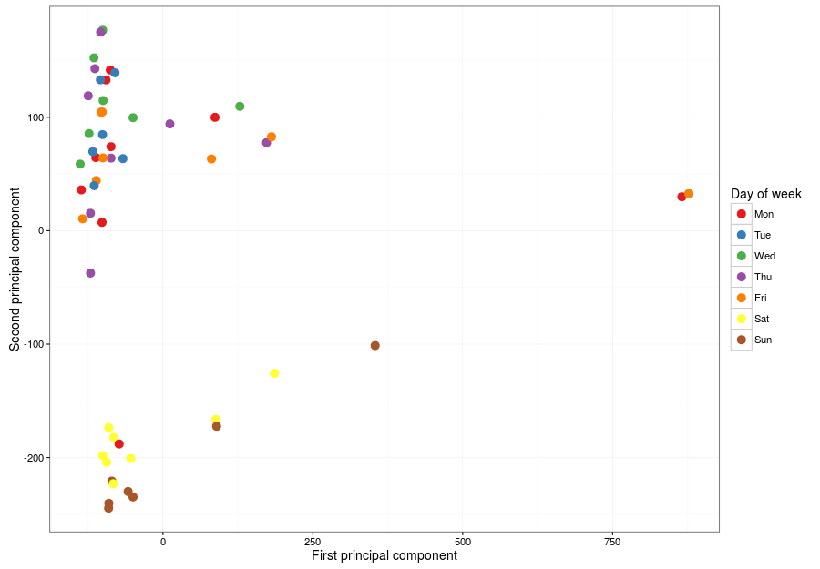
Which is very good. There are (at least) two very distinctive behaviours: one for week days (top left) and one for weekends (bottom left). There are two weird days (right) that I will check now, along with that offending Monday mixed with the weekends, which I suspect belonged to a long weekend. Let's check right now, beginning with those outliers to the right.
# Check the "offending days"
# Add the day to have a proper reference
pcares$day <- bixipca$day
pcares[pcares$pc1 > 750, ]
        pc1      pc2 day_of_week        day
57 834.1724 15.75442         Mon 2015-11-16
58 847.5419 18.44485         Tue 2015-11-17
61 847.5419 18.44485         Fri 2015-11-20
62 847.5419 18.44485         Sat 2015-11-21
63 847.5419 18.44485         Sun 2015-11-22
It turns out there are five days, not only two, but four of them overlap perfectly. Remember those days that produced NAs in my data and we removed them? November 18th and 19th were there. And now the rest of the days from that week show up. Why? Let's do a quick plot of data in those days, just to see what is happening.
plot(bixidata[bixidata$day == "2015-11-16", -1])
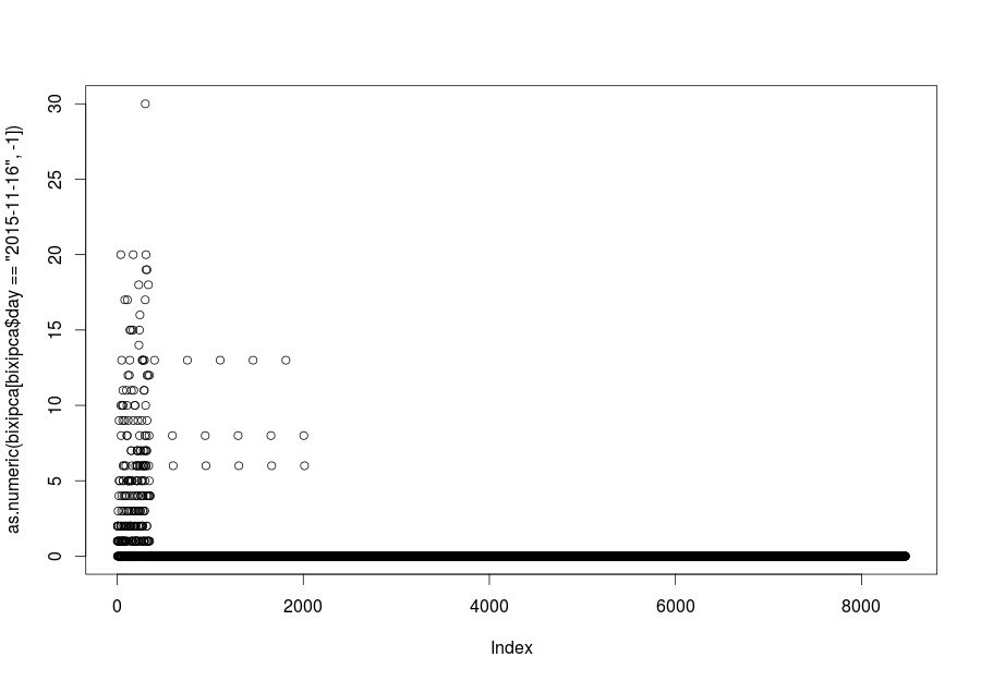
Remember that I told you that Bixi stops its service on November 15th? Well, we selected just too many days of data when we truncated our dataset for th first time. Luckily for us, the PCA plot came to tell us that we were doing something wrong.
What about the weird Monday?
pcares[pcares$day_of_week == "Mon" & pcares$pc2 < -100, ]
         pc1       pc2 day_of_week        day
22 -105.3991 -186.4822         Mon 2015-10-12
October 12th, 2015, Thanksgiving here in Canada.
Now, I could check the typical, distinctive patterns that distinguish weekdays from weekends, but I want to do something different. Instead, let's see what the pattern for each base says about different geographical areas.
Are there residential / business patterns in the data?
This is something I found when I was analyzing Madrid's data: some bases show the pattern one would expect from a residential area (stations get empty during the day and populated at night) and some what you would expect from zones where people go to work (stations get populated during work hours and get empty during the night, when people return home). Let's see if we can find the same thing here.
For starters, after all we have seen, I am going to truncate our dataset once more: let's get a single week of data, but a complete one. From looking at all the data points I had to remove previously, it seems that almost anything in October that does not include the 9th is going to be OK (and let's skip the 12th also, remember the holiday above), so let's settle for the time window that goes between 2015-10-19 and 2015-10-25, Monday to Sunday.
bixi <- bixi[bixi$filedate >= as.POSIXct("2015-10-19 00:00:00") &
             bixi$filedate < as.POSIXct("2015-10-26 00:00:00"), ]
Ok, and now I am going to try to check which bases are in residential areas and which are in business areas. For the residential area, I am going to pick "Rachel/Des Érables". For the business area, "Union/René Lévesque". These are a bit arbitrary selections based on my (imperfect) knowledge of the city, but let's see if they match our intuition:
sset1 <- bixi[bixi$name == "Rachel/Des Érables", ]
sset2 <- bixi[bixi$name == "Union/René Lévesque", ]
total <- rbind(sset1, sset2)
plt2 <- ggplot(total, aes(x = filedate, y = nbBikes)) +
        geom_line(aes(color = name)) +
        scale_color_manual(values = c("red", "blue"), name = "Base") +
        scale_x_datetime(date_breaks = "1 day") +
        xlab("Time") + ylab("Available bikes at station")
print(plt2)
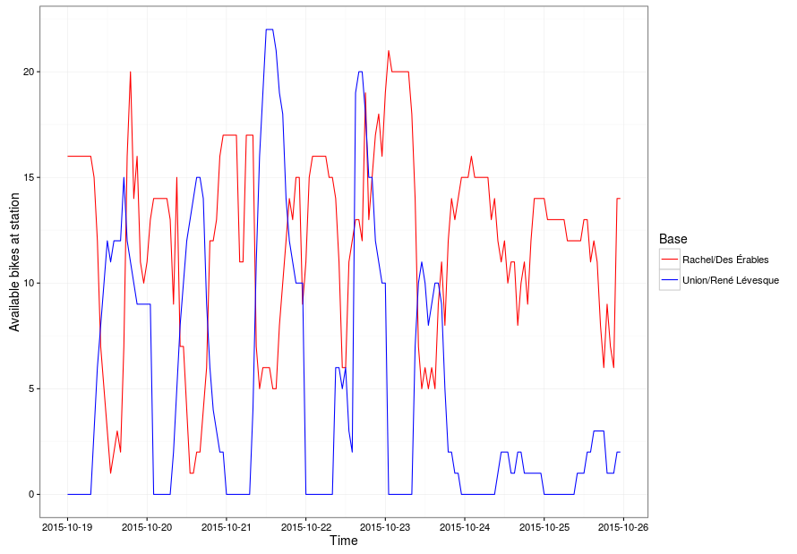
It looks good: the bike pattern in our residential station bottoms during the day, and is crowded at night, and the other one looks shows a completely opposed behavior. So let's do the following: using these two bases as initial seeds, let's compute how each other station correlates with them. If something correlates more than 0.2 with one of them, let's call that residential or business, respectively. Otherwise, let's label it as unknown. I know I have chosen a very low correlation threshold, but the data is noisy and I only want this label for plotting purposes. Bear with me, we are close to the end.
scores <- bixi %>%
    group_by(name) %>%
    summarise(residential_score = cor(nbBikes, sset1$nbBikes),
              business_score = cor(nbBikes, sset2$nbBikes))

scores$status <- ifelse(scores$residential_score > 0.2, "Residential",
                        ifelse(scores$business_score > 0.2, "Business", "Unknown"))

bixi <- left_join(bixi, scores)
Now, what if we plot a given hour on a map?
library(ggmap)
# Plot data for a single day, just to test
testdata <- bixi[bixi$filedate == as.POSIXct("2015-10-19 12:00:00"), ]
mymap <- get_map(location = make_bbox(long, lat, bixi),
                 source = "osm", maptype = "roadmap")
ggmap(mymap) + geom_point(data = testdata, aes(x = long, y = lat, color = status,
                                               size = nbBikes), alpha = 0.5) +
    scale_color_manual(values = c("red", "darkgreen", "#0000ee"), name = "Base type") +
    scale_size_area(name = "Number of available bikes") +
    geom_text(data = testdata, x = -73.535, y = 45.432, aes(label = filedate),
              size = 5)
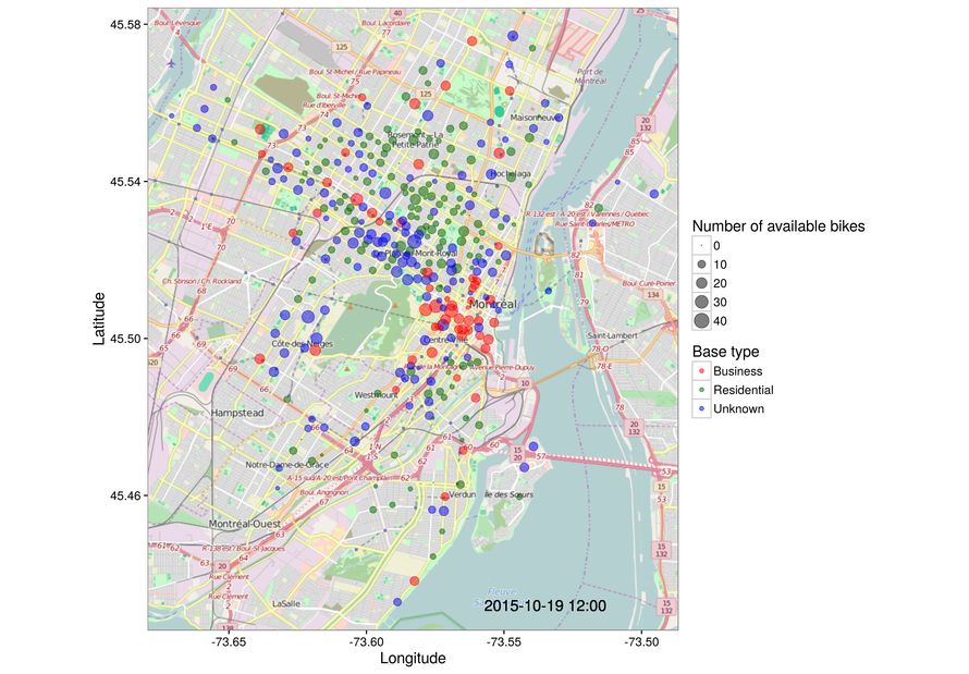
That's very good! The stations that we thought would be in business areas tend to appear near downtown, Square Victoria and the surrounding streets. Residential bases are far from there, near Le Plateau and surrounding neighborhoods. And the ones we could not identify are a bit in between, which probably means those stations do not show only one of the proposed behaviors and can be quite mixed in their usage patterns. Also, please consider that this is at best a subset of all the available Bixi stations, as we have dropped a few along the way. In any case, so far, so good.
But this is a single, static point in time. We'll now try to make the whole thing dynamic. To spare you a bit of pain (this is getting long already, isn't it?), I will tell you that I tried following this guide quite closely but I was getting an odd error when the referenced library calls the convert command to generate the GIF file. In the end I modified things a bit in order to use this:
# Let's assume we already have mymap, so we don't have to request it every time.
draw_bases <- function(timepoint) {
    testdata <- bixi[bixi$filedate == as.POSIXct(timepoint), ]
    timepointstr <- strftime(timepoint, "%Y-%m-%d %H:%M")
    plt_dyn <- ggmap(mymap) +
               geom_point(data = testdata, aes(x = long, y = lat, color = status,
                                               size = nbBikes), alpha = 0.5) +
               scale_color_manual(values = c("red", "darkgreen", "#0000ee"), name = "Base type") +
               scale_size_area(name = "Number of available bikes") +
               geom_text(data = testdata, x = -73.535, y = 45.432, aes(label = timepointstr),
                         size = 5) +
               xlab("Longitude") + ylab("Latitude")
    ggsave(plt_dyn, filename = paste0("/tmp/", timepointstr, ".png"))
    #print(plt_dyn)
}

draw_animation <- function() {
    times <- unique(bixi$filedate)
    lapply(times, draw_bases)
}
It is the same function structure that should be used with saveGIF, but here I am saving individual PNG files to the temporary folder in order to later call convert directly from the command line to assemble the final animation. I am saving the PNG files at full resolution, so I could create a hi-res animation in another format if needed to. For now, I just had to call draw_animation() and wait till all the static frames have been saved. And then I open a terminal and run:
# Resize each frame so it is easier to generate the final gif (my computer complained
# too much before I tried this)
for png in *.png; do echo "$png" && convert -resize 1000 -format gif "$png" "$png".gif; done
# GIF with endless loop and 0.5 seconds between frames
convert -delay 50 -loop 0 2015-10-*.gif bixi_1.gif
And here we have the glorious final result: how Montrealers moved using their bikes for one week during 2015. You can see perfectly how people go to work in the mornings and return to their homes in the evening. Here is a local copy of the GIF file if you'd rather download it from my server.
This is the end of the tour. I hope you had fun (I did), and I also hope that this post helps you understand that data analysis is not something you simply do flawlessly in a perfect dataset, or in one from which you know all the caveats in advance. A lot of the work is exploratory, and when you think the exploratory phase has finished and you start to do some actual work, then you find that there were tricks hidden around each corner.
You can find the complete R file used for this analysis in this Github repository. I am not re-distributing the original XML files I downloaded as I don't know if I have permission to do so (but I'll ask). Also, remember that I have published the files to all the data analysis projects that have appeared on this blog here.